Recurrent Depth: Why Repeating the Same Transformer Layers Can Help
A Transformer reads text as tokens. A token can be a word, part of a word, or punctuation. Each token starts with an embedding, a list of numbers representing it. Layers update these numbers using information from the text. This changing list of numbers is called the hidden state.
The weights, also called parameters, are learned numbers that control these updates. When the model writes an answer, the weights stay fixed while the hidden state changes. Think of the weights as rules and the state as the information they work on.
A standard, fixed-depth Transformer passes this state through a fixed sequence of layers. A recurrent-depth Transformer, also called a looped Transformer, reuses one layer, or a group of layers, several times before producing the output.
The idea is to let the model do more work without adding a new set of weights for every extra step. One pass means running the whole repeated block once.
What are a layer, a block, and a pass?
A Transformer layer usually contains two main parts:
Self-attention
      ↓
Feed-forward network (MLP)
      ↓
Updated hidden state
Self-attention lets each token use information from other tokens. In a model that predicts the next token, it can use itself and earlier tokens, but not future ones. The feed-forward network, also called an MLP (multilayer perceptron), then processes the numbers for each token.
The sketch leaves out two operations inside the layers:
Residual connections add a calculated update to the existing state. If the state is [10, 20] and the update is [2, -3], the result is [12, 17]. This lets a layer learn changes to its input rather than having to recreate the whole state. It also helps gradients travel backward during training, explained later.
Normalization rescales the hidden-state numbers to keep their size easier to control across repeated calculations. It does not make all the numbers equal or turn them into probabilities.
Both happen inside the layers. They are not extra passes through the block.
People often use layer and block to mean the same thing. Here is the distinction in this article:
- Layer: one Transformer layer, as described above.
- Recurrent block: one layer or a group of layers that the model reuses.
- Pass: running the entire recurrent block once, with its layers running in order.
For a three-layer block:
Pass 1: input → L1 → L2 → L3 → updated state
Pass 2: updated state → L1 → L2 → L3 → next state
That is two passes and six layer executions. L1, L2, and L3 have their own weights, but each layer reuses its weights on the next pass. The whole group repeats, not just the last layer.
The problem it tries to solve
One way to give a Transformer more computation is to make it deeper:
Input → L1 → L2 → L3 → L4 → L5 → L6 → OutputThese six layers normally have six different sets of weights. Adding more layers means storing more weights, which takes more memory.
A looped model can use fewer layers and run them more than once:
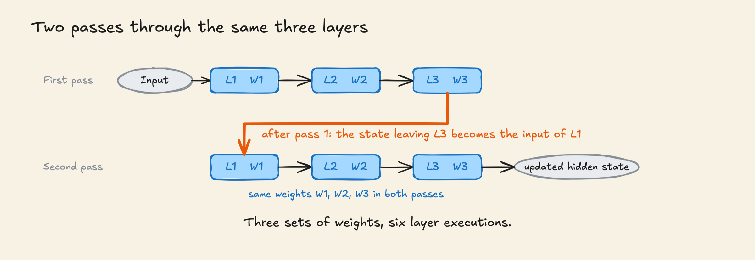
Three layers run twice, using the same weights on both passes. That gives six layer steps while storing only three sets of weights.
The two models are still different. Six separate layers can learn six different ways to process their input. The looped model has to reuse the same three.
Where does the loop happen?
A looped model does not always repeat the entire network. A common design has three parts:
Opening layers
      ↓
Repeated middle block
      ↓
Closing layers
The middle block, or core, runs several times with the same weights. The opening layers process the token embeddings. After the loop, the closing layers process the final state, and the output head turns it into probabilities for the next token.
Here is our three-layer example inside the full model:
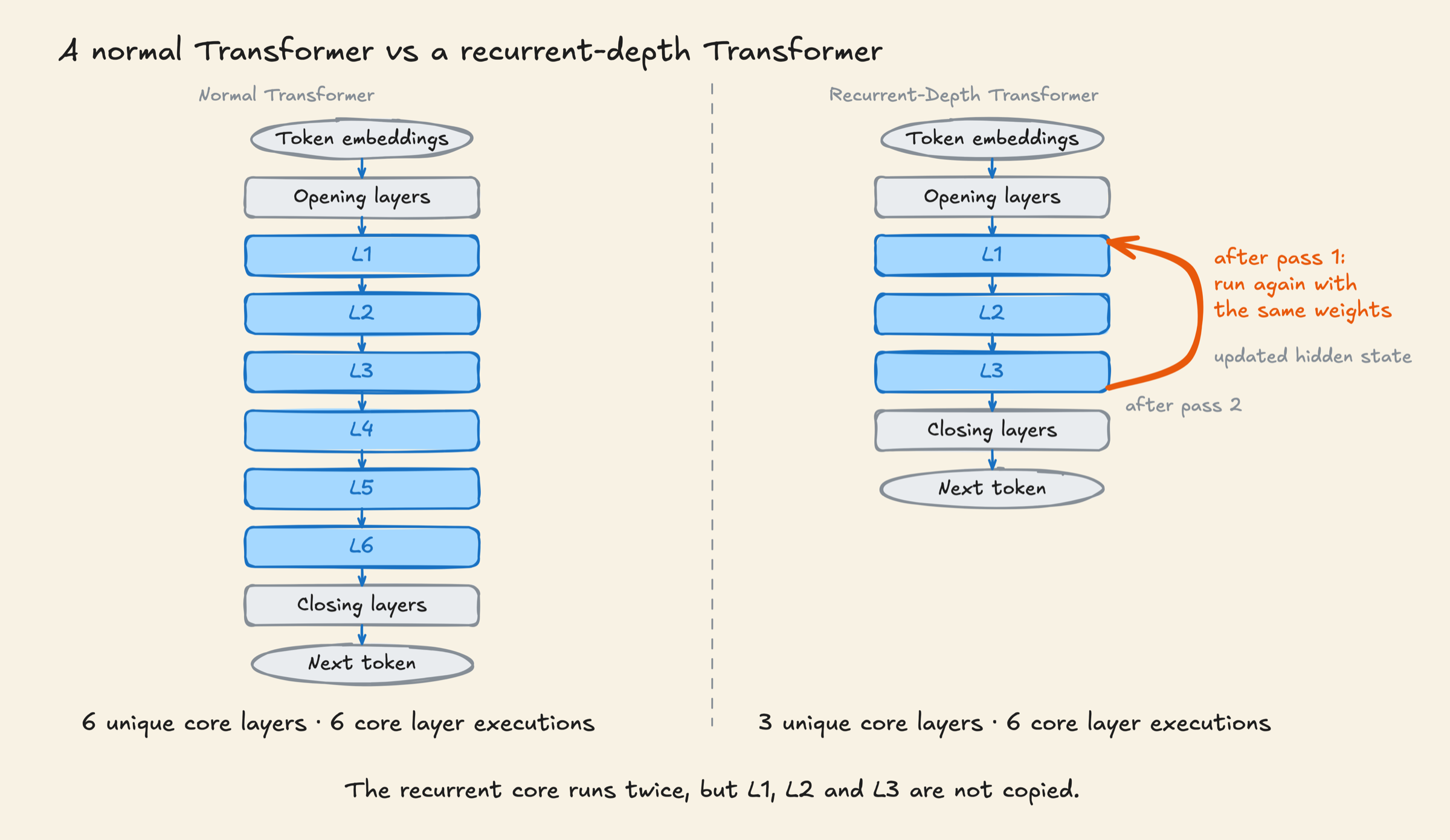
In this example, the core runs twice before the model chooses a token. It does not write a complete answer and then read it again:
Current token representations
          ↓
Repeated block: first pass
          ↓
Repeated block: second pass
          ↓
Output probabilities
          ↓
Next token
After choosing a token, the model adds it to the text and processes it to predict the next one. Another loop runs, but the model does not have to recalculate everything for earlier tokens: it can keep their attention information in a KV cache, explained below. The extra steps happen inside the network before a token is chosen, which is why this is recurrence in depth.
Running a trained model is called inference. The work it does while answering is called test-time compute.
A real model can use different layer and pass counts. Geiping et al. (2025) built a 3.5-billion-parameter model with 2 opening layers, a 4-layer core, and 2 closing layers. With 32 passes through that core, it runs 2 + 4 × 32 + 2 = 132 layer steps using eight different layers. This counts steps, not separate layers with their own weights. Model design, section 3
Why can the same block produce a different result?
Each pass works on the result of the previous pass, so its input can change.
Let F stand for the whole repeated block and h0 for its starting state. Here are three passes. Each F means one pass through all the layers in the block:
h1 = F(h0)
h2 = F(h1)
h3 = F(h2)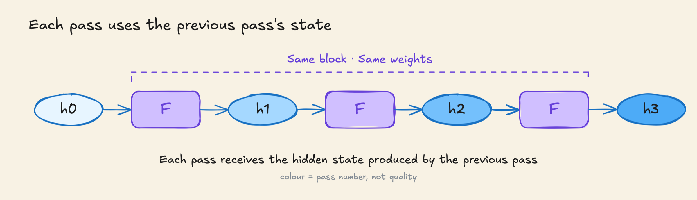
Later passes use the same F on the state produced by the previous pass. The result can change, though it does not have to change on every pass.
For example, suppose we repeat this function:
F(x) = (x + 100) / 2Starting with x = 0:
Pass 1: F(0)    = 50
Pass 2: F(50)   = 75
Pass 3: F(75)   = 87.5
The same function gives a different result each time. These results approach 100 because of the function we chose. A model's next pass could help, make no difference, or make the answer worse.
A Transformer works with vectors, or lists of numbers. Its hidden state may contain thousands of numbers per token.
Why give every pass the same input information?
The Geiping model gives each pass two things:
- e: input information. The opening layers produce it from the text once, before the loop. It stays the same throughout that loop.
- h: the working state. It starts as random numbers, h0, and each pass produces an updated version.
The same e is used alongside the latest h:
h1 = F(e, h0)
h2 = F(e, h1)
h3 = F(e, h2)
F(e, h) means the block uses both inputs. It joins their lists of numbers, then uses a learned transformation to mix them back into one list of the original size before running the core layers. This mixing step also uses the same weights on every pass. It does not replace h with e or reset the work. Model design, sections 3.1 and 3.2
The model keeps e separately and reads it again on every pass. Updating h does not overwrite e.
To see what this means, reuse our earlier averaging example, but now supply 100 as a separate input, e. For easy arithmetic, choose h0 = 0 rather than a random starting value:
Stored input: e = 100
Update rule: new h = (e + previous h) / 2

Pass 1 reads e = 100 and h0 = 0
Produces h1 = (100 + 0) / 2 = 50

Pass 2 reads e = 100 and h1 = 50
Produces h2 = (100 + 50) / 2 = 75

Pass 3 reads e = 100 and h2 = 75
Produces h3 = (100 + 75) / 2 = 87.5
Pass 2 receives both 100 and 50, not just 50. It does not have to recover the original input from the previous result because e is still available separately.
The actual model combines lists of numbers using learned weights, not this averaging rule. The example only shows how a fixed input and a changing state can be used together.
Keeping e separate means h is not the only place that must preserve the input information.
This supports repeated updates that still depend on the input. It does not by itself guarantee that the state settles down or that the answer is correct. Other looped models may handle the input and starting state differently.
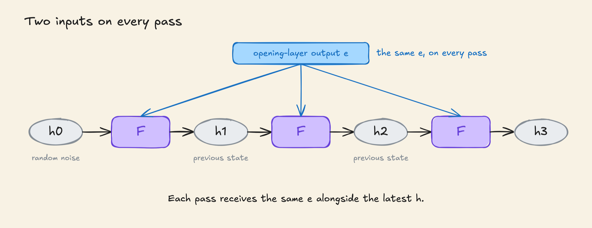
This describes one loop. When processing a new token, the opening layers prepare its e. In the basic Geiping setup, its working state starts from fresh random numbers, while cached attention information from earlier tokens remains available. The paper also tests reusing the previous token's final state instead. Neither approach means keeping one e unchanged for the entire answer. State reuse, section 6.3
Why can another pass improve the answer?
Each pass can use information worked out during an earlier pass.
Consider this question:
A warehouse has 3 shelves. Each shelf holds 4 boxes. Each box contains 5 parts. How many parts are there?
Here is one way to picture how later passes could use earlier results:
After initial processing:
the state holds information about shelves, boxes and parts

After a later pass:
it could combine 3 shelves × 4 boxes per shelf = 12 boxes

After another pass:
it could use those 12 boxes × 5 parts per box = 60 parts

Final output:
60 parts
These are imagined steps, not observations inside the model. A hidden state contains numbers, not instructions such as "now multiply 3 by 4."
“60 parts” is the completed answer shown for illustration, not necessarily a single output token.
Using one operation's result as the input to another is called composition. Ordinary deep Transformers do this too. In a looped model, some of these operations use the same weights.
More passes help only if the model has learned to do useful work with them.
Can more passes help with larger problems?
Fan et al. (2024) studied whether a model could solve problems with longer inputs than it saw during training. This is called length generalization. One task was parity: checking whether a string of 0s and 1s contains an odd or even number of ones. Another was binary addition, which uses only the digits 0 and 1.
Their model predicts the full answer after the loop, rather than one token at a time. Training sets the pass count by input length. Models trained on inputs of 1 to 19 bits did well on longer inputs with enough passes.
These results came from specific tasks and training methods. We cannot assume that giving any model more passes will let it solve longer questions. Fan et al., sections 3 to 6
The model must be trained for recurrence
Simply repeating layers in an ordinary pretrained Transformer is unlikely to work well. After another pass, the hidden state may look quite different from anything those layers saw during training.
A recurrent-depth model is trained with the loop in place, either from the start or through further training called fine-tuning. The block learns to update a state that it will process again.
How many layers and how many passes?
These are separate choices. The number of layers in the core is part of the model's design. The number of passes says how often that same core runs. A diagram with 32 pass positions does not mean 32 separate blocks with their own weights.
The Geiping model has a four-layer core. During training, its pass count is sampled randomly, averaging roughly 32. During inference, the count can be set in advance or controlled by a stopping rule, described below. It need not match a particular training run. Model design and training
How does training change the shared weights?
Training has three stages:
- Forward calculation: run the passes, produce a prediction, and compare it with the correct next token to calculate an error score, called the loss. The training text provides that correct token. The hidden state changes between passes, but the weights stay fixed throughout this calculation.
- Backward calculation: trace the calculation backward to work out how small changes to each weight would affect the loss. This is backpropagation. The resulting numbers are called gradients.
- Weight update: an optimizer, the rule used to adjust weights, uses those gradients to make an update intended to reduce the loss.
A gradient is not a corrected answer sent backward. It tells us how sensitive the loss is to a weight. Backpropagation calculates these effects through the connected operations; it does not run the model in reverse to recover the input. Backpropagation basics
Because the same weights are used repeatedly, the backward calculation adds together contributions from their different uses. There is one shared set to update, not a separate set for each pass. The model does not update its weights after pass 1 and then use new weights in pass 2.
During ordinary inference, only the forward calculation runs. There is no training loss, backpropagation, or weight update.
A small example of one shared weight learning
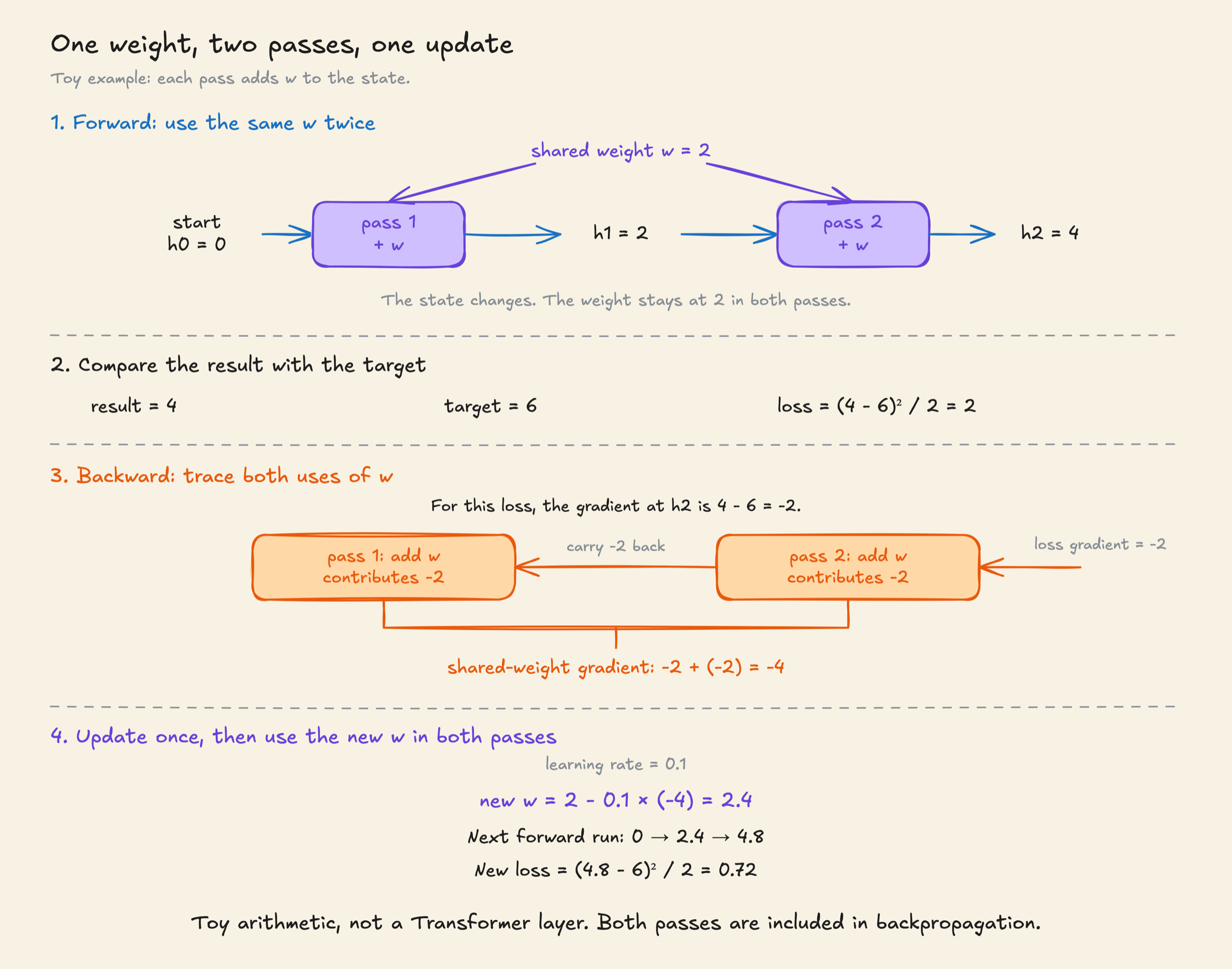
Suppose a toy block simply adds one weight w to its input. Use it twice, starting with h0 = 0 and w = 2. We want the final result to be 6:
Forward:
Pass 1: h1 = h0 + w = 0 + 2 = 2
Pass 2: h2 = h1 + w = 2 + 2 = 4

Target: 6
Loss: (h2 - target)² / 2 = (4 - 6)² / 2 = 2
The loss and the gradient are different numbers. The loss measures the error. The gradient tells us how the loss would change if the result changed slightly. For this particular loss formula, the gradient at h2 is h2 - target, or 4 - 6 = -2. The negative sign means that slightly increasing the result would reduce the loss. The loss itself is still 2.
Now trace the two uses of w backward:
- Pass 2: adding a little more w raises h2 by that same amount. This use contributes a gradient of -2.
- Pass 1: adding a little more w raises h1. Pass 2 carries that increase into h2. This use also contributes -2.
Both uses belong to the same weight, so their contributions add to -4. Choose a learning rate of 0.1. This multiplies the gradient to control the size of the weight update:
Update the shared weight once:
new w = old w - learning rate × gradient
      = 2 - 0.1 × (-4)
      = 2.4

Run both passes again with the updated weight:
Pass 1: h1 = 0 + 2.4 = 2.4
Pass 2: h2 = 2.4 + 2.4 = 4.8
New loss: (4.8 - 6)² / 2 = 0.72
The weight increased by 0.4, from 2 to 2.4, and the loss fell from 2 to 0.72. Both passes now use 2.4; neither has its own weight. This toy example traces backward through both passes. A Transformer has many weights and uses a different prediction loss, but shared weights still collect contributions from their uses in the backward calculation.
Why stop the backward calculation early?
Backpropagation needs intermediate results from the forward calculation, called activations. Sharing weights does not make these results identical: each pass processes a different state. Keeping results for a long chain of passes takes memory, and tracing backward through that chain takes work.
The Geiping model runs backward through at most the last eight passes. This is truncated backpropagation through time. Here, the repeated steps are in depth, not across tokens. It saves memory for retained activations and limits backward work, but gives an incomplete gradient because earlier steps are left out. Every forward pass still costs computation. Training method, section 3.3
Eight is this experiment's training choice, not a rule for recurrent models. With 32 forward passes, the last eight are 25 to 32. With 40, they are 33 to 40. The boundary moves with the forward pass count. If there are fewer than eight passes, the backward calculation can cover them all.
Reading the 32-pass training diagram
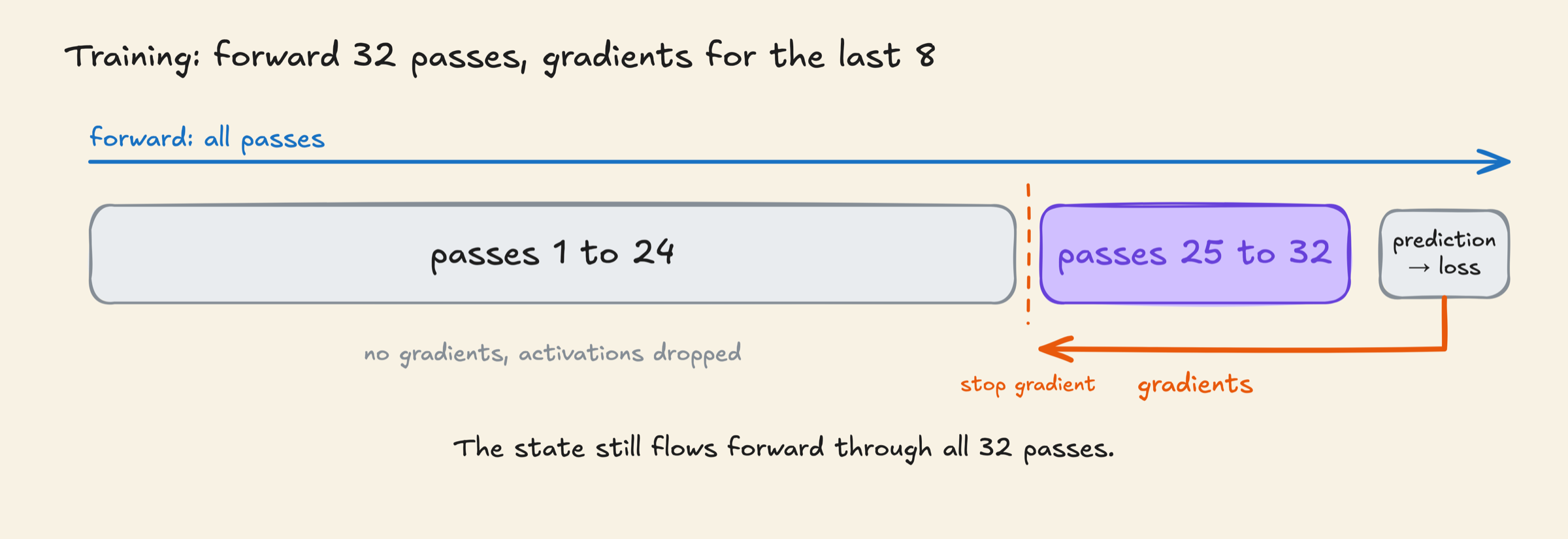
For this example, follow the diagram in this order:
- Grey, passes 1 to 24: each pass updates the state and sends it onward. Their internal results are not kept for backpropagation. The output of pass 24, h24, is still passed to pass 25.
- Purple, passes 25 to 32: the forward calculation continues, now retaining the results needed for backpropagation.
- After pass 32: the closing layers produce the prediction and training calculates the loss. The box on the right represents prediction and loss.
- Orange arrow, backward: the calculation starts from that loss, goes through the closing layers, then through passes 32, 31, 30, 29, 28, 27, 26 and 25. That is eight passes, including pass 32.
- Dashed boundary: h24 is treated as a fixed input to this backward calculation. It does not trace how passes 1 to 24 produced h24.
“No gradients” in the grey region does not mean those passes use untrained weights. They share the weights used in the purple region, so the later weight update changes the block used everywhere. What is missing is the gradient contribution through the earlier passes, not their forward work.
The opening layers can still learn too: their output e feeds the retained passes directly, so gradients can reach them through that route. Stopping the backward chain at h24 does not cut this separate connection.
What it saves and what it does not
Reusing layers lets the model run more steps with fewer weights. It still has to do the work on every pass.
It helps to separate three kinds of memory discussed here:
| What is stored? | Why keep it? | What do extra passes change? |
|---|---|---|
| Weights | The learned numbers used by the layers | The core reuses the same set. |
| Saved activations | Intermediate results needed for backpropagation | More tracked passes need more saved results. Truncation limits this. |
| KV cache | Attention information reused when processing later tokens | Separate entries for more passes take more space. Reusing slots limits this. |
These are different savings. Limiting training activations does not limit the inference KV cache, and sharing weights does not make either one free. This is not a complete list of everything stored during training.
Running a block twice uses the same stored weights, but does the work twice. Producing an answer usually takes longer.
Too many passes can also make answers worse. Some models control how much each pass changes the state. Others use a stopping rule to decide when enough passes have run.
How does the model know when to stop?
Universal Transformers (Dehghani et al., 2018) learn a stopping rule for each token position. Some positions can stop while others get more passes. This is called adaptive computation time. Their design is different from the Geiping model.
The Geiping paper tests another rule. After a pass, the model sends the current state through the closing layers and output head to calculate a probability for each possible next token. These probabilities describe what token might come next, given the text so far. They are not scores for whether the whole answer is correct. Calculating them does not select or write a token yet. Model code
For example, suppose the text ends with “The capital of France is”. Treat Paris and Lyon as single tokens in this simplified example:
| Possible next token | After pass 4 | After pass 5 |
|---|---|---|
| Paris | 80% | 81% |
| Lyon | 10% | 9% |
| All other tokens combined | 10% | 10% |
These are made-up numbers. They show how predictions can change between passes, not a measured result from the model. The stopping rule compares the full list of token probabilities, not just the most likely token or the three grouped rows above.
If the loop continues, the next core pass uses the working state from the previous core pass, not these probabilities. Unlike the fixed-count example earlier, this method runs the output path for intermediate checks too, which takes extra computation.
KL divergence measures how much those probabilities differ between passes. When it falls below 0.0005, the experiment stops the loop and chooses a token. That cutoff belongs to this experiment, not all models. A maximum pass count can also stop the loop if the predictions keep changing. Stopping experiment, section 6.1, stopping implementation
The threshold is a cutoff for change, not a benchmark score or a confidence percentage. A benchmark is a set of test tasks used to evaluate model performance; it is not consulted to make this stopping decision. The made-up probabilities above do not establish that the 0.0005 cutoff has been met.
This rule checks whether the token probabilities have changed very little, not whether the hidden state has stopped changing. A prediction that stays the same can still be wrong.
Why can memory still grow if weights are shared?
Attention saves keys and values for earlier tokens in a KV cache. Keys help find relevant information, and values hold the information used. Saving these numbers avoids calculating them again for every new token.
Even with the same weights, each pass can produce different keys and values because the hidden state has changed. If the model keeps a separate cache for each pass, more passes need more cache memory.
For the same input length, 32 passes need 32 times as much core cache memory as one pass if every pass has its own cache. The opening and closing layers add their entries only once. The model's total memory does not grow by the same factor because the stored weights stay the same.
Early stopping raises another question. If token A stops after pass 4, what does a later token B read when it reaches pass 5? A has no pass-5 entry. The Geiping method uses A's deepest available cached version, from pass 4 in this example, rather than recalculating the missing pass. Missing cache entries, remark 6.1
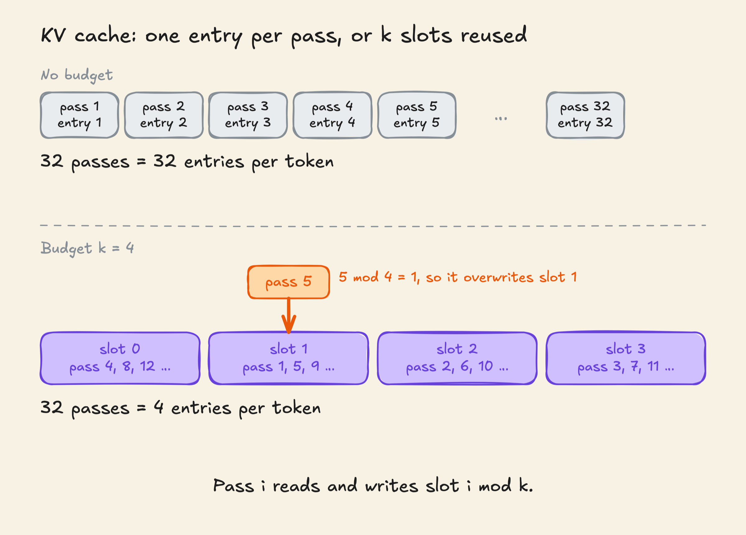
Cache memory can also be limited deliberately. Geiping et al. keep only k cache slots. Pass i reads and writes slot i mod k, where mod means the remainder after division. Later passes overwrite earlier slots. Here, an entry was calculated but replaced, rather than never calculated because of early stopping.
For a small example, use four slots and stop after five passes. Follow the cached information for just one token, A:
After A's pass 1:
slot 1 holds A's keys and values from pass 1

After A's pass 5:
slot 1 holds A's keys and values from pass 5
A's pass-1 version has been replaced

When a later token B runs pass 1:
it reads slot 1 for earlier tokens
for A, that slot now contains the pass-5 version
Each token has its own entries within these slots. Writing B's information does not delete A's information. What is replaced is an earlier pass's version for the same token. If A ran more passes, slot 1 could be replaced again at pass 9, then 13, and so on.
This saves space by keeping fewer versions, not by storing all versions in a smaller box. Attention may now use information from a different pass than it would with separate caches. The paper found this worked well in its tests, but it is not a guarantee of identical predictions or unchanged quality on every task. Cache sharing, section 6.2
Can we see what happens inside the loop?
Some models write intermediate steps, called a chain of thought. Recurrent depth allows extra work on the hidden state before the next token. This is called latent reasoning, where intermediate results stay as numbers inside the model.
Input → hidden state → repeated block → updated hidden state → output tokenThose numbers are harder to follow than written steps. Ordinary Transformers also use hidden states, and even written reasoning does not reveal every internal calculation.
In short
A looped Transformer uses the same weights again on the state from its last pass:
h0 → F → h1 → F → h2 → F → h3Each pass can use what an earlier pass worked out. The model needs training to make use of this. Extra passes do not add more weights, but they do take more computing work and time.
Check your understanding: if our three-layer core runs ten times instead of twice, what changes?
It still stores three sets of weights, but runs 30 layer steps instead of six. Separate caches would need more memory too. Whether the answers improve needs testing.
References
Universal Transformers Dehghani, Gouws, Vinyals, Uszkoreit, Kaiser. The original shared-layer Transformer. One block runs again and again, with adaptive computation time to halt each position on its own. https://arxiv.org/abs/1807.03819
Looped Transformers as Programmable Computers Giannou, Rajput, Sohn, Lee, Lee, Papailiopoulos. Shows that a looped 13-layer Transformer with fixed weights can run programs: a calculator, basic linear algebra, and in-context learning with backpropagation. The input sequence holds both the instructions and the memory. https://arxiv.org/abs/2301.13196
Scaling up Test-Time Compute with Latent Reasoning: A Recurrent Depth Approach Geiping, McLeish, Jain, Kirchenbauer, Singh, Bartoldson, Kailkhura, Bhatele, Goldstein. The 3.5B model used as the example in this article: 2 + 4 + 2 layers, a random number of passes during training, and a KL-divergence stopping rule. https://arxiv.org/abs/2502.05171
Looped Transformers for Length Generalization Fan, Du, Ramchandran, Lee. Tests whether models trained on short inputs can solve longer ones with more passes. The tasks include parity, copying and binary addition. The model predicts the full answer after the loop. https://arxiv.org/abs/2409.15647